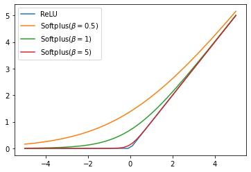
ReLU is one of the commonly used activations for artificial neural networks, and softplus can viewed as its smooth version.
ReLU ( x ) = max ( 0 , x ) softplus β ( x ) = 1 β log ( 1 + e β x ) , \text{ReLU}(x) = \max(0, x) \ \ \ \ \ \ \ \ \ \ \ \text{softplus}_\beta(x) = \frac{1}{\beta}\log(1 + e^{\beta x}), ReLU ( x ) = max ( 0 , x ) softplus β ( x ) = β 1 log ( 1 + e β x ) , where β \beta β β \beta β
Dombrowski et al. (2019) 's Theorem 2 says that for one-layer neuron network with ReLU activations g ( x ) = max ( 0 , w T x ) g(x) = \max(0, w^Tx) g ( x ) = max ( 0 , w T x ) g β ( x ) = softplus β ( w T x ) g_\beta(x) = \text{softplus}_\beta(w^Tx) g β ( x ) = softplus β ( w T x )
E ϵ ∼ p β [ ∇ g ( x − ϵ ) ] = ∇ g β / ∥ w ∥ ( x ) . \mathbb{E}_{\epsilon \sim p_\beta}[\nabla g(x - \epsilon)] = \nabla g_{\beta/\|w\|} (x). E ϵ ∼ p β [ ∇ g ( x − ϵ ) ] = ∇ g β / ∥ w ∥ ( x ) . The gradient wrt. to the input of the softplus network is the expectation of the gradient of the ReLU network when the input is perturbed by the noise ϵ \epsilon ϵ
In the following, I state the proof that is provided in the supplement of the paper .
Let assume for a moment that x x x E ϵ ∼ p β [ g ( x − ϵ ) ] = softplus β ( x ) \mathbb{E}_{\epsilon \sim p_\beta} [ g(x-\epsilon) ] = \text{softplus}_\beta(x) E ϵ ∼ p β [ g ( x − ϵ ) ] = softplus β ( x )
softplus β ( x ) = ∫ − ∞ ∞ p ( ϵ ) g ( x − ϵ ) d ϵ , (1) \text{softplus}_\beta(x) = \int_{-\infty}^{\infty} p(\epsilon) g(x-\epsilon) \text{d}\epsilon \tag{1}, softplus β ( x ) = ∫ − ∞ ∞ p ( ϵ ) g ( x − ϵ ) d ϵ , ( 1 ) where p ( ϵ ) p(\epsilon) p ( ϵ )
σ β ( x ) = ∫ − ∞ ∞ p ( ϵ ) 1 [ x − ϵ > 0 ] d ϵ = ∫ − ∞ x p ( ϵ ) d ϵ . \begin{aligned} \sigma_\beta(x) &= \int_{-\infty}^{\infty} p(\epsilon) \mathbb 1_{[x-\epsilon > 0]} \text{d}\epsilon \\ &= \int_{-\infty}^{x} p(\epsilon) \text{d}\epsilon. \end{aligned} σ β ( x ) = ∫ − ∞ ∞ p ( ϵ ) 1 [ x − ϵ > 0 ] d ϵ = ∫ − ∞ x p ( ϵ ) d ϵ . Applying another differentiaion yields
β ( e β ϵ / 2 + e − β ϵ / 2 ) 2 ⏟ ≜ p β ( x ) = p ( x ) . \underbrace{\frac{\beta}{(e^{\beta \epsilon /2} + e^{-\beta \epsilon / 2})^2}}_{\triangleq p_\beta(x)} = p(x). ≜ p β ( x ) ( e β ϵ / 2 + e − β ϵ / 2 ) 2 β = p ( x ) . Substituting p β p_\beta p β
softplus β ( x ) = ∫ − ∞ ∞ p β ( ϵ ) g ( x − ϵ ) d ϵ = E ϵ ∼ p β [ g ( x − ϵ ) ] . (2) \begin{aligned} \text{softplus}_\beta(x) &= \int_{-\infty}^{\infty} p_\beta(\epsilon) g(x-\epsilon) \text{d}\epsilon \\ &= \mathbb{E}_{\epsilon \sim p_\beta} [ g(x-\epsilon)]. \tag{2} \end{aligned} softplus β ( x ) = ∫ − ∞ ∞ p β ( ϵ ) g ( x − ϵ ) d ϵ = E ϵ ∼ p β [ g ( x − ϵ ) ] . ( 2 ) Consider x , ϵ ∈ R d \mathbf x, \mathbf \epsilon \in \Reals^d x , ϵ ∈ R d p β ( ϵ ) = ∏ i = 1 d p β ( ϵ i ) p_\beta(\mathbf \epsilon) = \prod_{i=1}^d p_{\beta}(\epsilon_i) p β ( ϵ ) = ∏ i = 1 d p β ( ϵ i ) ϵ \mathbf \epsilon ϵ d d d
ϵ = ϵ p w ^ + ∑ i = 1 d ϵ 0 ( i ) w 0 ^ ( i ) , \mathbf \epsilon = \epsilon_p \hat{\mathbf w} + \sum_{i=1}^d \epsilon_0^{(i)} \hat{\mathbf{w}_0}^{(i)}, ϵ = ϵ p w ^ + i = 1 ∑ d ϵ 0 ( i ) w 0 ^ ( i ) , s.t. ∀ i ∈ [ d ] , w ^ T w 0 ^ ( i ) = 0 \forall i \in [d], \hat{\mathbf w}^T \hat{\mathbf{w}_0}^{(i)} = 0 ∀ i ∈ [ d ] , w ^ T w 0 ^ ( i ) = 0 w = ∥ w ∥ w ^ \mathbf w = \| \mathbf w \| \hat{\mathbf{w}} w = ∥ w ∥ w ^
E ϵ ∼ p β [ g ( x − ϵ ) ] = E ϵ ∼ p β [ ReLU ( w T ( x − ϵ ) ) ] = E ϵ ∼ p β [ ReLU ( w T x − w T ϵ ) ] = E ϵ ∼ p β [ ReLU ( w T x − ϵ p ∥ w ∥ ) ] . \begin{aligned} \mathbb{E}_{\epsilon \sim p_\beta} [ g(\mathbf x- \mathbf \epsilon)] &= \mathbb{E}_{\epsilon \sim p_\beta} [ \text{ReLU}(\mathbf w^T(\mathbf x- \mathbf \epsilon))] \\ &= \mathbb{E}_{\epsilon \sim p_\beta} [ \text{ReLU}(\mathbf w^T\mathbf x- \mathbf w^T \mathbf \epsilon)] \\ &= \mathbb{E}_{\epsilon \sim p_\beta} [ \text{ReLU}(\mathbf w^T\mathbf x- \epsilon_p \| \mathbf w \|)]. \end{aligned} E ϵ ∼ p β [ g ( x − ϵ ) ] = E ϵ ∼ p β [ ReLU ( w T ( x − ϵ ) ) ] = E ϵ ∼ p β [ ReLU ( w T x − w T ϵ ) ] = E ϵ ∼ p β [ ReLU ( w T x − ϵ p ∥ w ∥ ) ] . Consider ϵ ~ ≜ ϵ p ∥ w ∥ \tilde{\mathbf \epsilon} \triangleq \mathbf \epsilon_p \| \mathbf w \| ϵ ~ ≜ ϵ p ∥ w ∥
E ϵ ∼ p β [ ReLU ( w T x − ϵ p ∥ w ∥ ) ] = ∫ − ∞ ∞ p β ( ϵ ) ReLU ( w T x − ϵ p ∥ w ∥ ) d ϵ = ∫ − ∞ ∞ p β ( ϵ ~ ∥ w ∥ ) ( 1 ∥ w ∥ ) ⏟ p β ∥ w ∥ ( ϵ ) ~ ReLU ( w T x − ϵ ~ ) d ϵ ~ = E ϵ ~ ∼ p β ∥ w ∥ [ ReLU ( w T x − ϵ ~ ) ] = softplus β ∥ w ∥ ( x ) . \begin{aligned} \mathbb{E}_{\epsilon \sim p_\beta} &[ \text{ReLU}(\mathbf w^T\mathbf x- \epsilon_p \| \mathbf w \|)] = \int_{-\infty}^{\infty} p_\beta(\mathbf \epsilon) \text{ReLU}(\mathbf w^T\mathbf x- \epsilon_p \| \mathbf w \|) \text{d} \mathbf \epsilon \\ &= \int_{-\infty}^{\infty} \underbrace{p_\beta\bigg(\frac{\tilde{\mathbf \epsilon}}{\| \mathbf w \|}\bigg) \bigg( \frac{1}{\| \mathbf w \|} \bigg)}_{p_\frac{\beta}{\|\mathbf w\|}(\tilde{\mathbf \epsilon)}} \text{ReLU}(\mathbf w^T\mathbf x- \tilde\mathbf{\epsilon}) \text{d} \tilde {\mathbf \epsilon} \\ &= \mathbb E_{\tilde{\mathbf \epsilon} \sim p_{\frac{\beta}{\| \mathbf w \|}}} [ \text{ReLU}(\mathbf w^T\mathbf x- \tilde\mathbf{\epsilon})] \\ &= \text{softplus}_{\frac{\beta}{\| \mathbf w \|}}(x). \end{aligned} E ϵ ∼ p β [ ReLU ( w T x − ϵ p ∥ w ∥ ) ] = ∫ − ∞ ∞ p β ( ϵ ) ReLU ( w T x − ϵ p ∥ w ∥ ) d ϵ = ∫ − ∞ ∞ p ∥ w ∥ β ( ϵ ) ~ p β ( ∥ w ∥ ϵ ~ ) ( ∥ w ∥ 1 ) ReLU ( w T x − ϵ ~ ) d ϵ ~ = E ϵ ~ ∼ p ∥ w ∥ β [ ReLU ( w T x − ϵ ~ ) ] = softplus ∥ w ∥ β ( x ) . Differentiating both sides yields the desired result. ◼️
(Visualization added on 02/06/2020)
Why does this result matter? In the paper, Dombrowski et al. (2019) show that attribution (explanation) maps can be arbitrarily manipulated. They argue that this is because the output manifold of the ReLU neural network has a large curvature, and it causes gradients wrt. to the input to be highly unstable when the input is slightly perturbed.
They show that one can prevent such manipulations by replacing ReLU with the softplus activation. Based on the theorem 2, they argue and empirically show that doing so has the same effect (attribution maps) as SmoothGrad, in which the attribution map is averaged from several maps of the input perturbed by some noise.
Reference Dombrowski et al. (2019) "Explanations can be manipulated and geometry is to blame"
Appendix From Softplus to Sigmoid Consider Softplus 1 ( x ) = log ( 1 + exp ( x ) ) \text{Softplus}_1(x) = \log(1+\exp(x)) Softplus 1 ( x ) = log ( 1 + exp ( x ) )
d d x Softplus 1 ( x ) = 1 1 + exp ( x ) exp ( x ) ⏟ Sigmoid ( x ) . \begin{aligned} \frac{\text{d}}{\text{d}x} \text{Softplus}_1(x) = \underbrace{\frac{1}{1+\exp(x)}\exp(x)}_{\text{Sigmoid}(x)}. \end{aligned} d x d Softplus 1 ( x ) = Sigmoid ( x ) 1 + exp ( x ) 1 exp ( x ) .