Conjugate Gradient 1

January 10, 2020
Table of Content

Steepest Gradient Descent
Residual and Error
Conjugate Directions
A-Orthogonal (Conjugacy)
Gram-Schmidt Conjugation
Summary: Conjugate Gradient Algorithm
Proofs

Othogonality of residual and search directions
Conjugate Gradient needs only n steps
Independency of residuals
Acknowledgements

Gradient is one the key ingredients when it comes to optimization. In some cases, one might employ second order methods, i.e. using Hessian; however, it is not common in machine learning to use such methods because we simply have too many variables.

In this article, I am going to talk about the conjugate gradient method for optimizing quadratic functions, i.e.

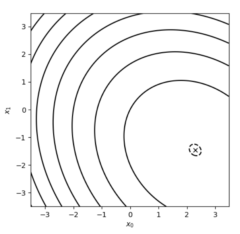
\begin{aligned} f(x) &= \frac{1}{2} x^TAx - b^Tx \\ x^* &= \underset{x}\text{argmin} f(x) \end{aligned}

where $A \in \mathbb{R}^{n\times n}$ is symmetric positive semi-definite and $b \in \mathbb{R}^n$ . $A$ and $b$ are coefficients of the functions. In this setting, the method ensures that we will converge to the solution within $n$ steps, where $n$ is the dimensions of variables.

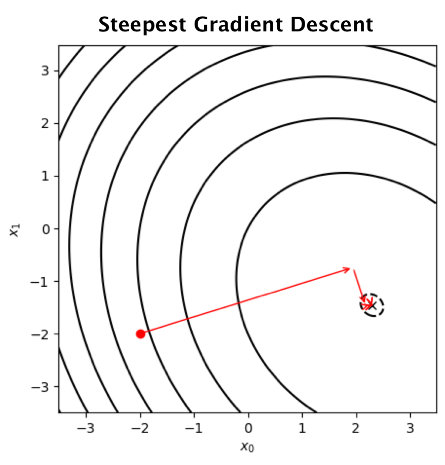
Steepest Gradient Descent

Let first revisit the gradient descent method. The method iteratively finds $f(x)$ 's possible minimizer $\hat x$ by using $x_{i+1} = x_i - \alpha_t \nabla f(x_i),$ where $\alpha_i$ is a learning rate at each iteration and $\nabla f(x_i)$ denotes $\nabla f(x)$ evaluated at $x_{i}$ . Noting that, in general, the gradient descent update does not guarantee that $\hat x = x^*$ , i.e. $\hat x$ might be at some local optima.

Naively, one can set $\alpha_i$ at some constate value, but a better way might be to choose the value based on the situation at hand. Consider performing a line search at each iteration to find the best value. In other word, we seek $\alpha_i$ by finding the first derivative at $f(x_{i+1})$ and set it to zero:

\begin{aligned} \frac{\partial}{\partial \alpha_i} \bigg|_{x=x_{i+1}} f(x) &= \nabla f(x_{i+1})^T \bigg( \frac{\partial}{\partial \alpha_i} x_i + \alpha_i \nabla f(x_i) \bigg) \\ &= \nabla f(x_{i+1})^T \nabla f(x_i) \\ &\overset{!}{=} 0. \\ \end{aligned}

This derivation tells us that, along the search direction $\nabla f(x_t)$ , the optimal value of $\alpha_t$ is the one leading to the location that two gradients are orthogonal. Solving the equation above for $\alpha$

\begin{aligned} \nabla f(x_{i+1})^T \nabla f(x_i) &= (Ax_{i+1} - b)^T\nabla f(x_i) \\ &= (A(x_i - \alpha \nabla f(x_i))-b)^T\nabla f(x_i) \\ &= (Ax_i - \alpha A \nabla f(x_i)-b)^T\nabla f(x_i) \\ &= (\nabla f(x_i) - \alpha A \nabla f(x_i))^T\nabla f(x_i) \\ \alpha &= \frac{\nabla f(x_i)^T \nabla f(x_i)}{\nabla f(x_i)^T A \nabla f(x_i)}. \end{aligned}

Residual and Error

Assume $x^*$ is known. Error at each step $e_t$ is

e_i = x^* - x_i,

which simply tells us how far we are from the answer. In contrast, residual at each step is the difference between the minimum value and our current value:

\begin{aligned} r_i &= b - Ax_i \\ &= Ax^* - Ax_i \\ &= Ae_i \end{aligned}

Combining the definitions of error and residual yields

\begin{aligned} r_i &= b - Ax_i \\ &= Ax^* - A x_i \\ &= A(x^* - x_i) \\ &= Ae_i. \end{aligned}

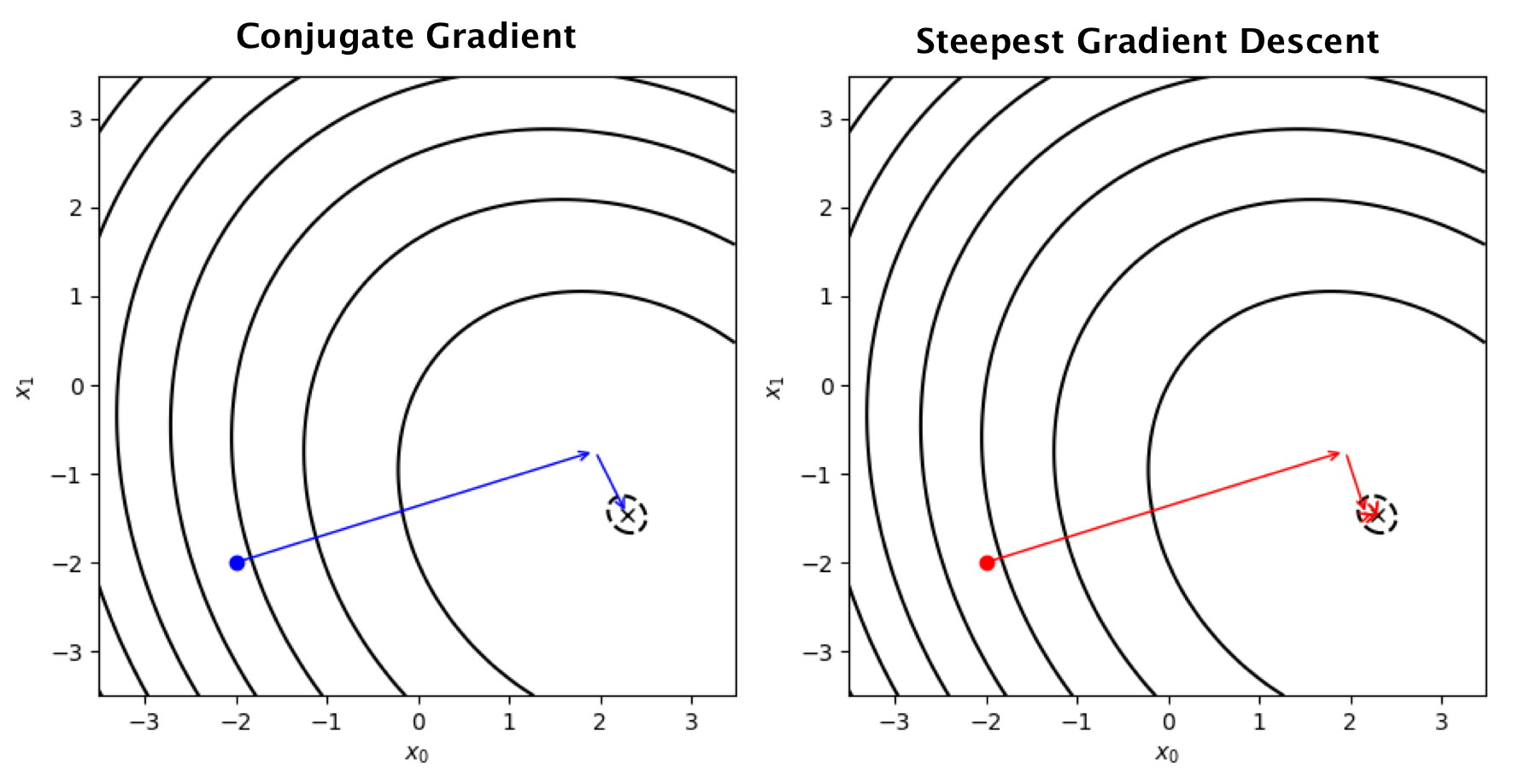
Conjugate Directions

One problem of Steepest Descent is that every move inteferes previous moves; hence slow convergence. It would be good to have search directions that do not affect each other.

Consider an update

x_{i+1} = x_i + \alpha_i d_i,

where $\alpha_i$ is update step and $d_i$ is a search direction. We can to find $\hat x$ in $n$ updates (using $n$ directions $d_1, \dots, d_n$ ), if these directions are orthogonal to each other

d_0 \perp d_1 \perp d_2 \perp \dots \perp d_n.

Therefore, the error at each step $e_t$ is also orthogonal to previous search directions, e.g.

\begin{aligned} e_1 &\perp d_0 \\ e_2 &\perp d_1 \perp d_0. \end{aligned}

Using this fact, we have

\begin{aligned} d_i^T e_{i+1} &= d_i^T(x^* - x_{i+1}) \\ &= d_i^T(x^* - (x_i + \alpha_i d_i)) \\ &= d_i^T(e_i - \alpha_i d_i) \\ &= 0 \end{aligned}

The derivation above yields $\alpha_i = \frac{d_i^T e_i}{d_i^T d_i}.$

A-Orthogonal (Conjugacy)

However, as we do not know $x^*$ so do $\alpha_i$ . Instead of requiring orthogonality $d_i^T d_j$ , we construct search directions that are orthogonal under the transformation of the matrix $A$ . In other word, we want $d_i$ and $d_j$ to be A-Conjugate (Orthogonal):

d_i^T A d_j = 0.

If we find the minimum along the search direction $d_i$ , we have

\begin{aligned} \frac{\partial}{\partial \alpha_i} f(x_{i+1}) &= \nabla f(x_{i+1})^T \bigg (\frac{\partial}{\partial \alpha_i} x_{i+1} \bigg ) \\ &= - r_{i+1}^T d_{i} \\ &= - (A e_{i+1})^T d_{i} \\ &\overset{!}{=} 0 \end{aligned}

Using this fact, we have

\begin{aligned} d_{i}^T A e_{i+1} &= d_i^T A (e_i - \alpha_i d_i) \\ &\overset{!}{=} 0 \\ \implies \alpha_i &= \frac{d_i^T A e_i}{d_i^T A d_i} \\ &= \frac{d_i^T r_i}{d_i^T A d_i}. \end{aligned}

Now, $\alpha_i$ is computable. By construction, taking the $\alpha_i d_i$ step ensures that $d_i^Tr_{i+1}=0$ . The only thing that we need to find is the set of A-conjugate search directions $\{d_i\}$ .

Gram-Schmidt Conjugation

Consider linearly independent vectors $u_0, u_1, \dots, u_{j-1}$ . One can construct A-orthogonal basis $\{d_0, d_1, \dots, d_{j-1}\}$ from these vectors using (Conjugate) Gram-Schmidt Process

d_j = u_j - \sum_{k=1}^{j-1} \beta_{jk} d_k,

where $\beta_{jk}$ is a scaling factor that we seek to find. One issue immediately arises: How should one construct $u_j$ ? It turns out that we can use $r_j$ as $u_j$ (Proof). Therefore, we have

d_j = r_j - \sum_{k=1}^{j-1} \beta_{jk} d_k. \tag{1}

Based on our conjugatecy requirement, this new direction $d_j$ should be A-orthogonal to all previous search directions $d_i$ for $i < j$ , hence

\begin{aligned} 0 \overset{!}{=} d_i^T A d_j &= d_i^TA ( r_j - \sum_{k=1}^{j-1} \beta_{jk} d_k ) \\ &= d_i^TA r_j - \sum_{k=1}^{j-1} \beta_{jk} d_i^T A d_k \\ &= d_i^TA r_j - \beta_{ji} d_i^T A d_i. \end{aligned}

Therefore, we have $\beta_{ji} = \frac{d_i^T A r_j}{d_i^T A d_i}.$

The derivation above shows how we construct A-orthogonal search directions. However, another problem is that the contruction uses all previous search directions in the process, hence large memory complexity. Fortunately, we can make this memory aspect more efficient.

Consider that $d_i ^T r_j = 0$ for $\forall i < j$ (Proof). Multiplying $r_{j}^T$ to Equation (1) yields

\begin{aligned} 0 \overset{!}{=}r_{j}^T d_i &= r_{j}^T \bigg( r_i - \sum_{k=0}^{i-1} \beta_{ik} d_k \bigg) \\ &= r_{j}^Tr_i - \sum_{k=0}^{i-1} \beta_{ik} \cancel{r_{j}^T d_k}. \\ \end{aligned}

Essentially, the derivation above tells us that $r_i^T r_j = 0, \forall i < j$ . Using this fact, one can derive

\begin{aligned} r_{i}^T r_{j+1} &= r_i^T (r_j - \alpha_jA d_j ) \\ &= r_i^T r_j - \alpha_j r_i^T A d_j. \end{aligned}

Because $r_i^T r_j = 0$ if $i \ne j$ ,

r_i^T A d_j = \begin{cases} \frac{1}{\alpha_i} r_i^T r_i &; \ \ i = j \\ - \frac{1}{\alpha_{i-1}} r_i^T r_i &; \ \ i = j + 1 \\ 0 &; \ \ \text{otherwise} \\ \end{cases}

Recall that $\beta_{ik} = \frac{r_i^T A d_k}{d_k^T A d_k}$ for $k = 0, \dots, i-1$ . Because $r_i^T A d_k = 0$ when $i > k+1$ , we have

\begin{aligned} d_i &= r_i - \sum_{k=0}^{i-1} \beta_{ik} d_k \\ &= r_i - \beta_{i,i-1} d_{i-1} \\ &= r_i + \underbrace{ \bigg( \frac{r_i^Tr_i}{\alpha_{i-1} d_{i-1}^T A d_{i-1}} \bigg) }_{\beta_i } d_{i-1}. \end{aligned}

Because $\alpha_{i-1} = \frac{d_{i-1}^Tr_{i-1}}{d_{i-1}A d_{i-1}}$ , we can derive

\begin{aligned} \beta_{i} &= \frac{r_{i}^Tr_{i}}{\alpha_{i-1} d_{i-1}^T A d_{i-1} } \\ &= \frac{r_{i}^T r_{i}}{d_{i-1}^Tr_{i-1}}. \end{aligned}

Using $d_i ^T r_j = 0, \forall i < j$ yields

\begin{aligned} d_{i} &= r_{i} + \beta_{i} d_{i-1} \\ r_i^T d_{i} &= r_i^T( r_{i} + \beta_{i} d_{i-1}) \\ &= r_i^Tr_{i} + \beta_{i} \cancel{r_i^T d_{i-1}} \end{aligned}

Therefore, we have

\beta_{i} = \frac{r_{i}^T r_{i}}{r_{i-1}^Tr_{i-1}}.

Summary: Conjugate Gradient Algorithm

Consider a random starting point $x_0$ and $r_0 = d_0 = -\nabla f(x_0)$ . The update step for the conjugate gradient algorithm contains

\begin{aligned} \alpha_i &= \frac{r_i^T r_i}{d_i^T A d_i} \\ x_{i+1} &= x_{i} + \alpha_i d_i \\ r_{i+1} &= r_i - \alpha_i A d_i \\ \beta_{i+1} &= \frac{r_{i+1}^T r_{i+1}}{r_{i}^Tr_i} \\ d_{i+1} &= r_{i+1} + \beta_{i+1} d_i \end{aligned}

Proofs

Othogonality of residual and search directions

We know that

\begin{aligned} e_1 &= e_0 - \alpha_0 d_0 \\ e_2 &= e_1 - \alpha_1 d_1 \\ &= e_0 - \alpha_0 d_0 - \alpha_1 d_1 \\ &\ \ \vdots \\ e_j &= e_0 - \sum_{k=0}^{j-1} \alpha_j d_j. \end{aligned}

Assume that $e_0 = \sum_{k=0}^{n-1} \delta_k d_k$ . Multiplying the equation by $d_j^TA$ yields

\begin{aligned} d_j^T A e_0 &= \sum_{k=0}^{n-1} \delta_k d_j^T A d_k \\ &= \delta_j d_j^T A d_j \\ \implies \delta_j &= \frac{d_j^T A e_0}{d_j^T A d_j} \\ &= \frac{d_j^T A (e_j + \sum_{k=0}^{j-1}(\alpha_k d_k))}{d_j^T A d_j} \\ &= \frac{d_j^T A e_j + \sum_{k=0}^{j-1}\alpha_k \cancel{d_j^T A d_k}}{d_j^T A d_j} \\ &= \frac{d_j^T r_j }{d_j^T A d_j} \\ &= \alpha_j. \end{aligned}

Hence,

\begin{aligned} e_j &= \sum_{k=0}^{n-1} \alpha_k d_k - \sum_{k=0}^{j-1} \alpha_k d_k \\ &= \sum_{k=j}^{n-1} \alpha_k d_k \end{aligned}

Consider $i < j$ and multiplying the equation above by $d_i^TA$ . We have

\begin{aligned} d_i^T A e_j &= \sum_{k=j}^{n-1} \alpha_k \cancel{d_i^T A d_k} \\ &= 0. \end{aligned}

Therefore, we prove that $d_i^T r_j = 0, \forall i < j$ . ■

Conjugate Gradient needs only n steps

Consider the following identity (from the previous proof)

\begin{aligned} e_j &= \sum_{k=0}^{n-1} \alpha_k d_k - \sum_{k=0}^{j-1} \alpha_k d_k. \end{aligned}

One can see that the error after $n$ step ( $e_n$ ) is zero. ■

Independency of residuals

From the Gram-Schmidt construction, we can show that

\begin{aligned} r_i &= d_i + \beta_i d_{i-1} \\ r_j^T r_i &= r_j^T(d_i + \beta_i d_{i-1}) \\ &= \cancel{r_j^Td_i} + \beta_i \cancel{r_j^T d_{i-1})} \\ &=0. \end{aligned}

■

Acknowledgements

This article is based on content from

Figures are made from Google Colab.